Analysis of Brexit Votes in 2016
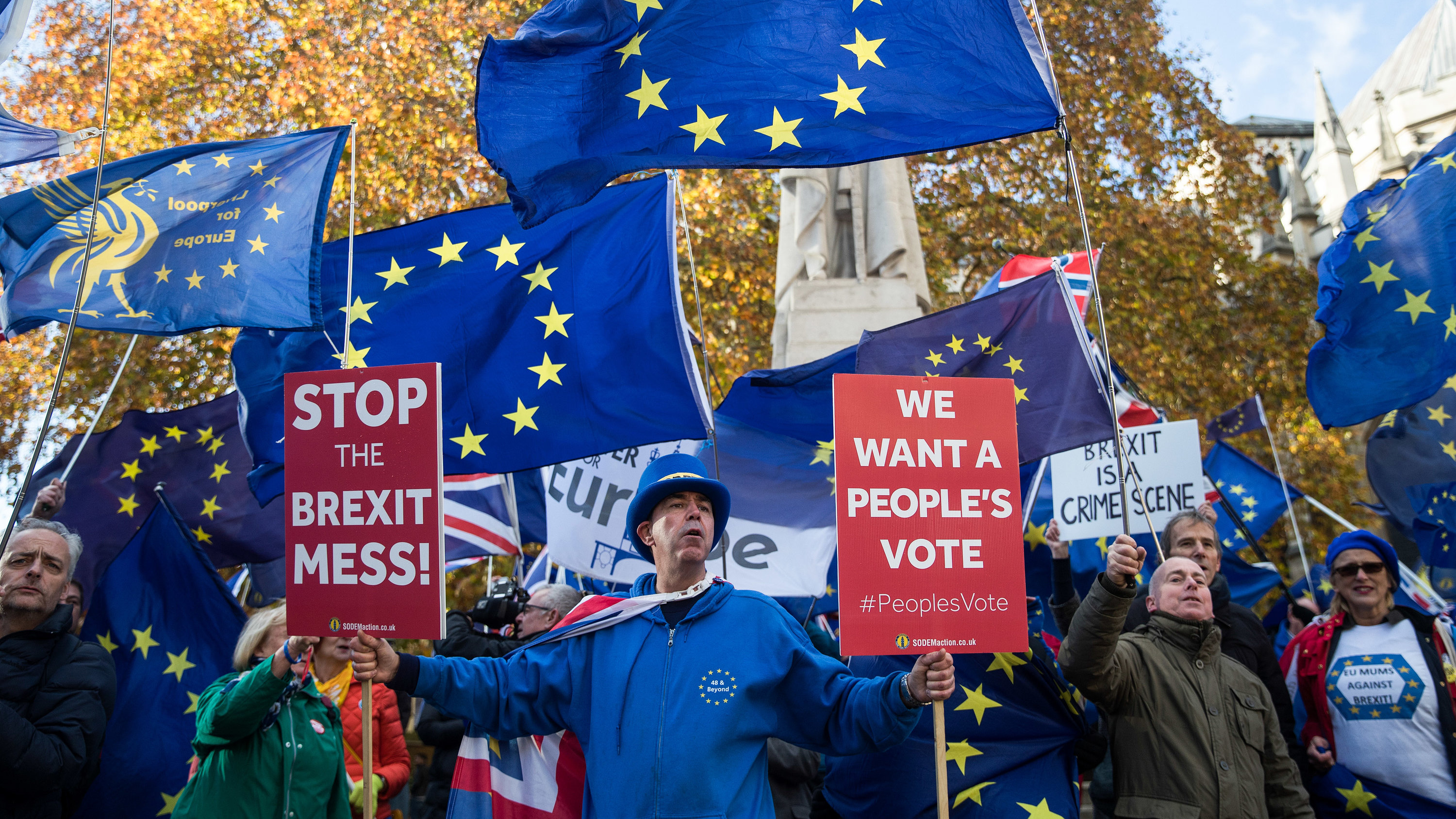
The political scene at UK was taken by a storm in 2016, when the entire population was out on the streets debating whether UK should exit the European Union or not. Once, the vote was conducted, we all know how it ended!
But, in this analysis we want to find out if the decision of the vote was influenced by certain factors.
Let’s have a look at the data first
glimpse(brexit)## Rows: 632
## Columns: 11
## $ Seat <chr> "Aldershot", "Aldridge-Brownhills", "Altrincham and Sale W…
## $ con_2015 <dbl> 50.6, 52.0, 53.0, 44.0, 60.8, 22.4, 52.5, 22.1, 50.7, 53.0…
## $ lab_2015 <dbl> 18.3, 22.4, 26.7, 34.8, 11.2, 41.0, 18.4, 49.8, 15.1, 21.3…
## $ ld_2015 <dbl> 8.82, 3.37, 8.38, 2.98, 7.19, 14.83, 5.98, 2.42, 10.62, 5.…
## $ ukip_2015 <dbl> 17.87, 19.62, 8.01, 15.89, 14.44, 21.41, 18.82, 21.76, 19.…
## $ leave_share <dbl> 57.9, 67.8, 38.6, 65.3, 49.7, 70.5, 59.9, 61.8, 51.8, 50.3…
## $ born_in_uk <dbl> 83.1, 96.1, 90.5, 97.3, 93.3, 97.0, 90.5, 90.7, 87.0, 88.8…
## $ male <dbl> 49.9, 48.9, 48.9, 49.2, 48.0, 49.2, 48.5, 49.2, 49.5, 49.5…
## $ unemployed <dbl> 3.64, 4.55, 3.04, 4.26, 2.47, 4.74, 3.69, 5.11, 3.39, 2.93…
## $ degree <dbl> 13.87, 9.97, 28.60, 9.34, 18.78, 6.09, 13.12, 7.90, 17.80,…
## $ age_18to24 <dbl> 9.41, 7.33, 6.44, 7.75, 5.73, 8.21, 7.82, 8.94, 7.56, 7.61…summary(brexit)## Seat con_2015 lab_2015 ld_2015 ukip_2015
## Length:632 Min. : 0.0 Min. : 0.0 Min. : 0.0 Min. : 0.0
## Class :character 1st Qu.:22.1 1st Qu.:17.7 1st Qu.: 3.0 1st Qu.: 9.2
## Mode :character Median :40.8 Median :31.2 Median : 4.6 Median :13.7
## Mean :36.6 Mean :32.3 Mean : 7.8 Mean :13.1
## 3rd Qu.:50.8 3rd Qu.:44.4 3rd Qu.: 8.6 3rd Qu.:17.1
## Max. :65.9 Max. :81.3 Max. :51.5 Max. :44.4
##
## leave_share born_in_uk male unemployed degree
## Min. :20.5 Min. :40.7 Min. :46.9 Min. :1.84 Min. : 5.1
## 1st Qu.:45.3 1st Qu.:86.4 1st Qu.:48.6 1st Qu.:3.23 1st Qu.:10.8
## Median :53.7 Median :92.5 Median :49.0 Median :4.19 Median :14.7
## Mean :52.1 Mean :88.2 Mean :49.1 Mean :4.37 Mean :16.7
## 3rd Qu.:60.2 3rd Qu.:95.4 3rd Qu.:49.4 3rd Qu.:5.21 3rd Qu.:19.6
## Max. :75.6 Max. :98.0 Max. :53.0 Max. :9.53 Max. :51.1
## NA's :59
## age_18to24
## Min. : 5.7
## 1st Qu.: 7.3
## Median : 8.3
## Mean : 9.3
## 3rd Qu.: 9.6
## Max. :32.7
## To get a sense of the spread, or distribution, of the data, we can plot a histogram, a density plot, and the empirical cumulative distribution function of the leave % in all constituencies.
# histogram
hist <- brexit %>%
  ggplot(aes(x = leave_share)) +
  geom_histogram(binwidth = 2.5) +
  theme_bw()

# density plot-- think smoothed histogram
dens <- brexit %>%
  ggplot(aes(x = leave_share)) +
  geom_density() +
  theme_bw()


# The empirical cumulative distribution function (ECDF)
dist <- brexit %>%
  ggplot(aes(x = leave_share)) +
  stat_ecdf(geom = "step", pad = FALSE) +
  scale_y_continuous(labels = scales::percent) +
  theme_bw()

final_plot <- (dist + dens + hist) +
  plot_annotation("Plots to Better Understand the Data Distribution")

final_plot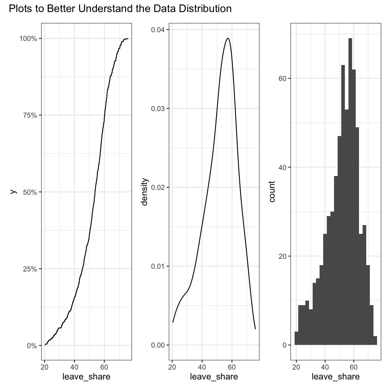
Were the voters born in UK?
One common explanation for the Brexit outcome was fear of immigration and opposition to the EU’s more open border policy. We can check the relationship (or correlation) between the proportion of native born residents in a constituency and its leave_share. To do this, let us get the correlation between the two variables
brexit %>%
  select(leave_share, born_in_uk) %>%
  cor()
## leave_share born_in_uk
## leave_share 1.000 0.493
## born_in_uk 0.493 1.000The correlation is almost 0.5, which shows that the two variables are positively correlated. It could be possible that those born in the UK, felt more national pride than the immigrants and also, wanted to preserve the identity of the UK as the ‘Land of the Brits’ and not have other nationalities flooding their society and take over their culture.
Was party affiliation the reason?
I believe it is also important to see if the political affiliations that the voters had affected the way they voted to leave the European Union or not.
# renaming the columns
brexit <- brexit %>%
  rename(Conservative = con_2015,
         Labour = lab_2015,
         LibDems = ld_2015,
         UKIP = ukip_2015)

# pivoting the table longer
brexit_longer <- brexit %>%
  pivot_longer(
    cols = Conservative:UKIP,
    names_to = "party",
    values_to = "count"
  )

color_party = c("#0087DC", "#E32636", "#FAA61A", "#6D3177") #assigning party colors to a vector

ggplot(brexit_longer,
  aes(
    x = count,
    y = leave_share
  )) +
  geom_point(aes(color = party), alpha = 0.4)  +
  scale_color_manual(values = color_party) +
  #adding trend lines
  geom_smooth(data = brexit,
      aes(x = Conservative, y = leave_share),
      color = color_party[1],
      method = "lm",
      se = TRUE) +
  geom_smooth(data = brexit,
      aes(x = Labour, y = leave_share),
      color = color_party[2],
      method = "lm",
      se = TRUE) +
  geom_smooth(data = brexit,
      aes(x = LibDems, y = leave_share),
      color = color_party[3],
      method = "lm",
      se = TRUE) +
  geom_smooth(data = brexit,
      aes(x = UKIP, y = leave_share),
      color = color_party[4],
      method = "lm",
      se = TRUE) +

  theme_bw() +
  theme(legend.position = "bottom") +
  theme(legend.title = element_blank()) +


  labs(
    title = "How political affiliation translated to Brexit Voting",
    x = "Party % in the UK 2015 General Elections",
    y = "Leave % in 2016 Brexit Referedum"
) 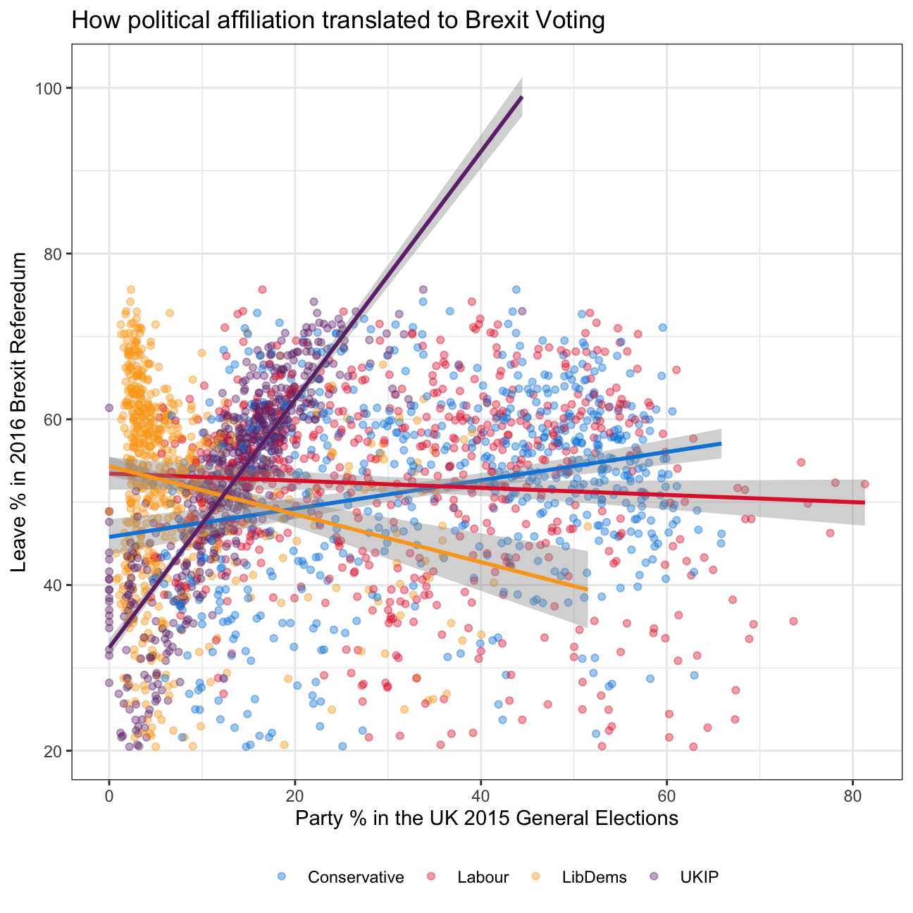
We plotted the percentage of those who voted to leave against the percentage of people with various party affiliations.
The plot showed that UKIP seemed to have a strong positive correlation. This aligns with their ideology of ‘Euroscepticism’. The party members were huge supporters of Brexit and hence, were one of the driving forces of encouraging the vote.